3D Ultrasound

Introduction
Background
Positioning
Verification of Accuracy
Mouse Pattern
Gyromouse
Lasermouse
Software Description
Downloads
Links

Introduction

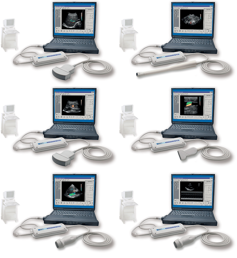
In my research we are currently investigating the use of 3D images. We use the Terason 2000 2D scanner system, an optical positioning system and a 3D rendering program called Sonocubic. This makes makes it possible to reconstruct correctly positioned 2D slices creating a 3D ultrasound image. The Terason scanner comes in a variety of versions with different scanner heads for different purposes.

Background

Our goal using 3D ultrasound images is to utilize the information redundancy that lies in adjacent 2D scanplanes. 3D ultrasound imaging also makes it easy for the user to visualize and understand the images. In this way it is easier to make a fast decision something that is critical in triage and emergency situations.

Positioning

Varying Offset

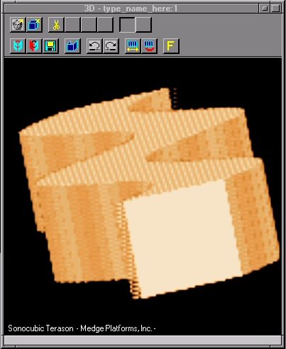
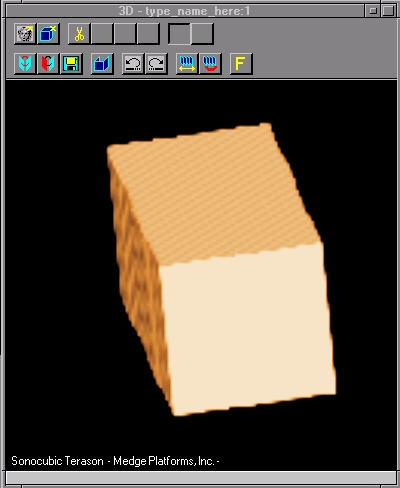
A comparison of the repositioning before and after compensation can be seen below. The images have been made by varying the position of the scanner and generating a computer generated ultrasound image with the content placed correctly as it would look if a real scan was performed.

The first example is a straight rod where the scanner is moved with a constant speed of 40 mm/sec while it is offset from the center path as a sine movement with a maximum offset of 40 mm.

Before offset correction		After offset correction

Varying Scanspeed and Offset

The next example is where both the scanner speed and the offset is varying. In order to visualize this it is necessary to use a four sided pyramid instead. Using this shape makes it possible to see both the variation in the scanspeed and the offset from the center scanpath.

Four different cases were considered :

Constant speed, no offset

Constant speed, variable offset

Variable speed, no offset

Variable speed, variable offset

A simulated scan was done for 2.5-3 seconds, covering a distance of approximately 120 mm. The corresponding positions were recorded and plotted (distance and offset). Below is the scanpath for the variable speed and variable offset.

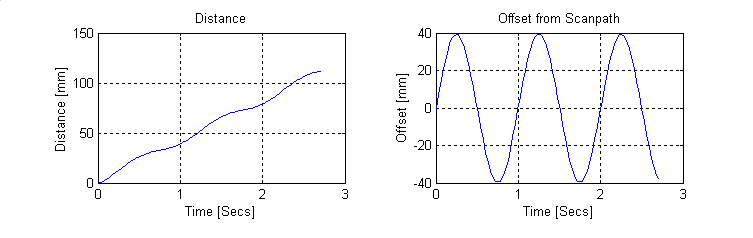
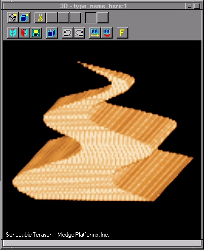
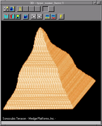
After generating the ultrasound images the reconstruction was done in Sonocubic. Below are some pictures that show how the compensation is working. The pictures were obtained by fooling Sonocubic giving it incorrect positioning information. In other words it is not a feature that can be added and removed after the scan has been obtained.

Before correction	After offset correction	After speed and offset correction

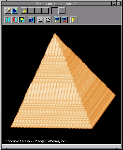As it can be seen the concept is working if the optical device can provide us with the correct positions.

Tube Test

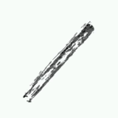
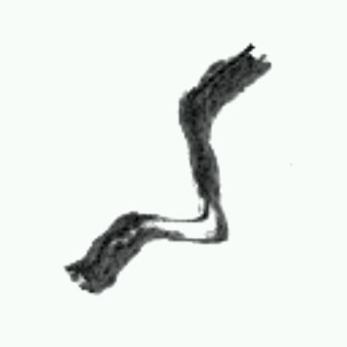
A test was done in real life with an ultrasound phantom containing tubes. The phantom was scanned from one end to the other with and without compensation. One big problem is that the optical tracking method is not very suited for even, smooth surfaces. It was therefore necessary to put some tape on top when the compensated dataset was recorded.

(Compensated pictures are on the left / uncompensated on the right)

Standard Sonocubic colors

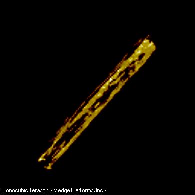
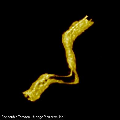
Gray - logarithmic inverted

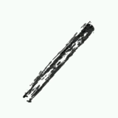
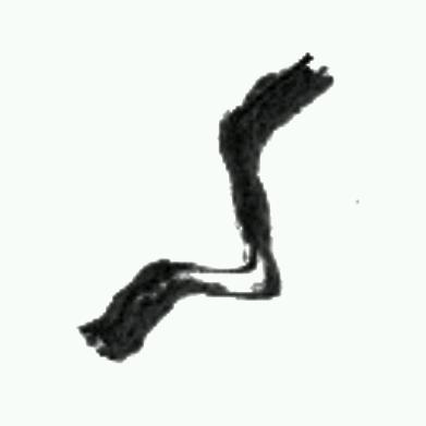
Gray - linear inverted

Verification of Accuracy

In order to see if the mouse is good enough a small experiment was carried out. The mouse was mounted in a socalled XY-recorder as shown in the picture below

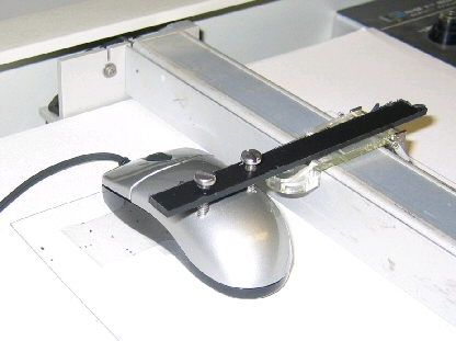
It was moved back and forth, first in the vertical direction, then in the horizontal direction and then in a slanted 45 degree angle. The positions from the mouse were recorded and a graph could be plotted.

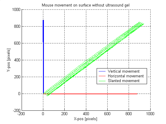
As it can be clearly seen in the slanted movement (green) the mouse did not track completely as expected. The reason for this lies in the mounting of it. The arm that holds the mouse is made of plastic and is relatively long. It therefore bends a little every time the mouse is moved in one direction or the other, and that is the reason for the spiralling curve.

Mouse Pattern

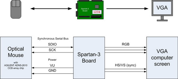
Here are some images that were captured from the optical sensor in the mouse. The idea behind this is to see if the image that is captured is in focus or not. The images are acquired using a Spartan FPGA and output directly to a computer monitor.

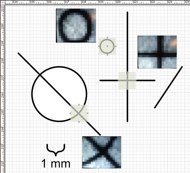
The pattern below was used as a test and the images in the shaded areas were captured. The images have 64 greyscales and a size of 18x18 pixels. Each pixel has a width or height of 25.4 mm/inch / 400 CPI = 0.0635 mm/pixel. This makes the CCD-array capture an area of (1.143 mm)^2 = 1.32 mm2 (in the figure below the captured images are enlarged!)